ggplot2 is also known as graph syntax, and it is a free, open-source, easy-to-use visualization package that is widely used in R. It is the most powerful visualization package written by Hadley Wickham.
It includes several layers to manage it. The layers are as follows:
The building blocks of a layer
The layers with variables of interest are as follows:
- Aesthetics: x-axis, y-axis, color, filling, size, label, alpha, shape, line width, line type
- Geometrics: Point, Line, Histogram, Bar Chart, Box Chart
- Facets: Columns, Rows
- Statistics: Binning, Smoothing, Descriptive, Intermediate
- Coordinates Coordinates: Cartesian, Fixed, Pole, Extreme
- Themes: Non-Data Links
data set
mtcars (Automotive Trend Car Road Test) includes fuel consumption as well as 10 aspects of car design and performance for 32 cars, and comes pre-installed with dplyr packaged in R.
# Installing the package
install.packages( "dplyr" )

# Loading package
library(dplyr)

# Summary of dataset in package
summary(mtcars)
Execute ggplot2 on the dataset
We designed the GGPLOT2 layer of the dataset containing 32 car brands and 11 attributes of the visualization MTCARS.
# Installing the package
install.packages( "ggplot2" )
# Loading packages
library(ggplot2)
library(dplyr)
# Data Layer
ggplot(data = mtcars)
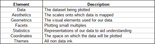
# Aesthetic Layer
ggplot(data = mtcars, aes(x = hp, y = mpg, col = disp))
# Geometric layer
ggplot(data = mtcars, aes(x = hp, y = mpg, col = disp)) + geom_point()
# Adding size
ggplot(data = mtcars, aes(x = hp, y = mpg, size = disp)) + geom_point()
# Adding color and shape
ggplot(data = mtcars, aes(x = hp, y = mpg, col = factor(cyl), shape = factor(am))) + geom_point()
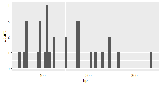
# Histogram plot
ggplot(data = mtcars, aes(x = hp)) +
geom_histogram(binwidth = 5 )
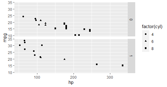
# Facet Layer
p < - ggplot(data = mtcars, aes(x = hp, y = mpg, shape = factor(cyl))) + geom_point()
# Separate rows according to transmission type
p + facet_grid(am ~ .)
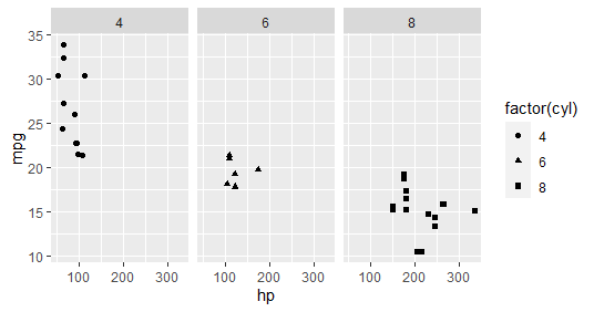
# Separate columns according to cylinders
p + facet_grid(. ~ cyl)
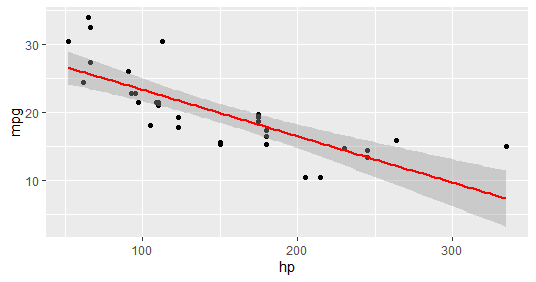
# Statistics layer
ggplot(data = mtcars, aes(x = hp, y = mpg)) +
geom_point() +
stat_smooth(method = lm, col = "red" )
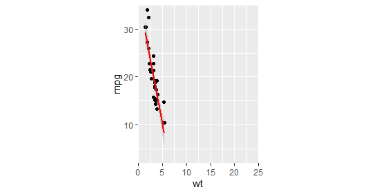
# Coordinates layer: Control plot dimensions
ggplot(data = mtcars, aes(x = wt, y = mpg)) +
geom_point() +
stat_smooth(method = lm, col = "red" ) +
scale_y_continuous( "mpg" , limits = c( 2 , 35 ), expand = c( 0 , 0 )) +
scale_x_continuous( "wt" , limits = c( 0 , 25 ), expand = c( 0 , 0 )) + coord_equal()
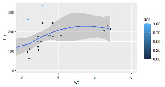
# Add coord_cartesian() to proper zoom in
ggplot(data = mtcars, aes(x = wt, y = hp, col = am)) +
geom_point() + geom_smooth() +
coord_cartesian(xlim = c( 3 , 6 ))
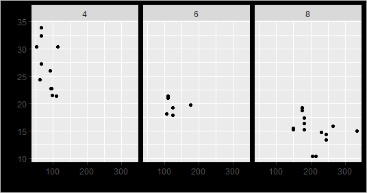
# Theme layer
ggplot(data = mtcars, aes(x = hp, y = mpg)) +
geom_point() + facet_grid(. ~ cyl) +
theme(plot.background = element_rect(
fill = "black" , colour = "gray" ))
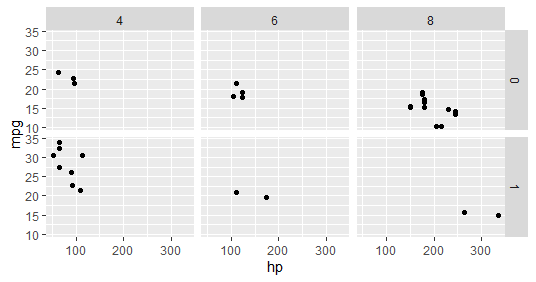
ggplot(data = mtcars, aes(x = hp, y = mpg)) +
geom_point() + facet_grid(am ~ cyl) +
theme_gray()The output is as follows:
Geometric layers
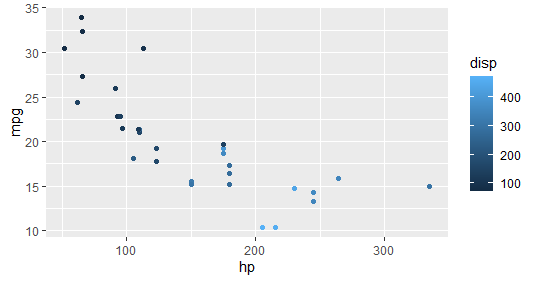
Geometry Layer – Add size
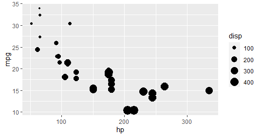
Geometry Layers – Add colors and shapes
Geometric Layers – Histogram
Facet Layer – Separate the rows according to the type of transport
Facet layer – columns separated according to the cylinder
Statistical layer
Coordinate Layer: Control chart size
Coord_cartesian() amplify appropriately
Topic layer – element_rect() function
Topic layer
ggplot2 offers various types of visualizations. You can use more parameters in the package because the package gives you more control over the visualization of the data. Many packages can be integrated with the ggplot2 package to make visualizations interactive and animated.