Stepwise development of deep convolutional neural networks to classify photos of dogs and cats
Dogs vs. The CATS dataset is a standard computer vision dataset that involves classifying photos as containing dogs or cats.
How does python identify cats and dogs? Although this problem sounds simple, it is only in recent years that deep learning convolutional neural networks have been used to effectively solve this problem. While effectively solving datasets, it can serve as a basis for learning and practicing how to develop, evaluate, and use convolutional deep learning neural networks from scratch for image classification.
This includes how to develop a powerful testing tool to estimate the performance of the model, how to explore improvements to the model, and how to save the model and load it later to make predictions on new data.
In this tutorial, you’ll learn how to develop a convolutional neural network to classify photos of dogs and cats.
By the end of this tutorial, you’ll know:
- How to load and prepare photos of dogs and cats for modeling.
- How to develop a convolutional neural network for photo classification from scratch and improve model performance.
- How to develop a photo classification model using transfer learning.
Start your project with my new book, Deep Learning for Computer Vision, including a step-by-step tutorial and a Python source code file for all the examples.
Let’s get started.
- October 2019 Update: Updated for Keras 2.3 and TensorFlow 2.0.
How to develop a convolutional neural network to classify photos of dogs and cats
Cohen Van der Velde photos, some rights reserved.
Tutorial overview
Prediction problems for dogs and cats
The Dog vs Cat dataset refers to the dataset used in the Kaggle Machine Learning Contest held in 2013.
The dataset consists of photos of dogs and cats and is available as a photo subset of a larger dataset of 3 million manually annotated photos. The dataset was developed as a partnership between Petfinder.com and Microsoft.
The dataset was originally used as a CAPTCHA (or fully automated public Turing test to distinguish between computers and humans), i.e., tasks that are considered trivial by humans but cannot be solved by machines, used on websites to distinguish between human users and bots. Specifically, the task is called “Asirra” or image recognition of animal species for restricted access, a CAPTCHA. This task was described in a 2007 article entitled “Asirra: A CAPTCHA that Exploits Interest-Aligned Manual Image Categolaization”.
We present Asirra, which is a CAPTCHA that asks users to identify cats from a set of 12 photos of cats and dogs. Asirra is easy for users; User studies have shown that humans can solve 99.6% of problems in less than 30 seconds. Unless there are significant advances in machine vision, we don’t expect a computer to solve it more than 1 in 54,000.
— Asirra: Captcha for manual image classification using interest alignment, 2007.
At the time of the competition’s release, state-of-the-art results were achieved using SVM and described in a 2007 paper titled “Machine Learning Attacks Asirra CAPTCHA” (PDF), which achieved 80% classification accuracy. It is this paper that proves that the task is no longer suitable for a CAPTCHA task shortly after it is proposed.
…… We describe a classifier that has an accuracy of 82.7% in distinguishing between images of cats and dogs used in Asirra. This classifier is a combination of support vector machine classifiers trained on color and texture features extracted from images. […] Our results suggest that Asirra should not be deployed without protection.
—Machine Learning Attack Asirra CAPTCHA, 2007.
Python Ways to Identify Cats and Dogs – The Kaggle contest offers 25,000 tagged photos: 12,500 dogs and the same number of cats. Predictions were then made on a test dataset of 12,500 unlabeled photos. Pierre Sermanet (currently a research scientist at Google Brain) won the contest and achieved a classification accuracy of about 98.914% on 70% of the subsamples of the test dataset. His approach was later described as part of a 2013 paper titled “OverFeat: Integrated Identification, Localization, and Detection Using Convolutional Networks.”
The dataset is easy to understand and small enough to fit into memory. As a result, it has become a great “hello world” or “starter” computer vision dataset for beginners when they are getting started with convolutional neural networks.
Therefore, it is routine to achieve approximately 80% accuracy using a manually designed convolutional neural network and to achieve more than 90% accuracy on this task using transfer learning.
Dog vs. cat dataset preparation
Categorizing photos of dogs and cats: This dataset can be downloaded for free from the Kaggle website, but I believe you must have a Kaggle account.
If you don’t have a Kaggle account, sign up first.
Download the dataset by visiting the Dogs vs. Cats Data page and click the “Download All” button.
This will download the 850 megabyte file “dogs-vs-cats.zip” to your workstation.
Unzip the file, and you’ll see train.zip, train1.zip, and a .csv file. Unzip train.zip file, as we will only focus on this dataset.
You will now have a folder called “train/” with 25,000 .jpg files for dogs and cats. Photos are tagged by file name with the words “dog” or “cat“. The file naming convention is as follows:
cat.0.jpg
...
cat.124999.jpg
dog.0.jpg
dog.124999.jpg
Draw pictures of dogs and cats
Feel free to look at a few photos in the catalog and you can see that they are all in color and vary in shape and size.
For example, let’s load and draw the first nine photos of a dog in one diagram.
A complete example is listed below.
# plot dog photos from the dogs vs cats dataset
from matplotlib import pyplot
from matplotlib.image import imread
# define location of dataset
folder = 'train/'
# plot first few images
for i in range(9):
	# define subplot
	pyplot.subplot(330 + 1 + i)
	# define filename
	filename = folder + 'dog.' + str(i) + '.jpg'
	# load image pixels
	image = imread(filename)
	# plot raw pixel data
	pyplot.imshow(image)
# show the figure
pyplot.show()
Run the example to create a graph that shows the top nine photos of dogs in the dataset.
As we can see, some of the photos are in landscape format, some are in portrait format, and some are square.
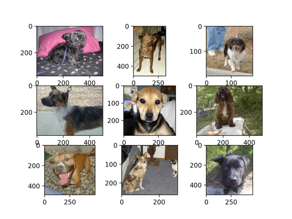
Diagram of the first nine photos of dogs in the Dogs vs Cats dataset
python recognition of cats and dogs example – we can update the example and change it to draw a cat photo; A complete example is listed below.
# plot cat photos from the dogs vs cats dataset
from matplotlib import pyplot
from matplotlib.image import imread
# define location of dataset
folder = 'train/'
# plot first few images
for i in range(9):
	# define subplot
	pyplot.subplot(330 + 1 + i)
	# define filename
	filename = folder + 'cat.' + str(i) + '.jpg'
	# load image pixels
	image = imread(filename)
	# plot raw pixel data
	pyplot.imshow(image)
# show the figure
pyplot.show()
Again, we can see that the photos are all different sizes.
We can also see a photo in which the cats are barely visible (bottom left) and another with two cats (bottom right). This suggests that any classifier suitable for this problem must be robust.
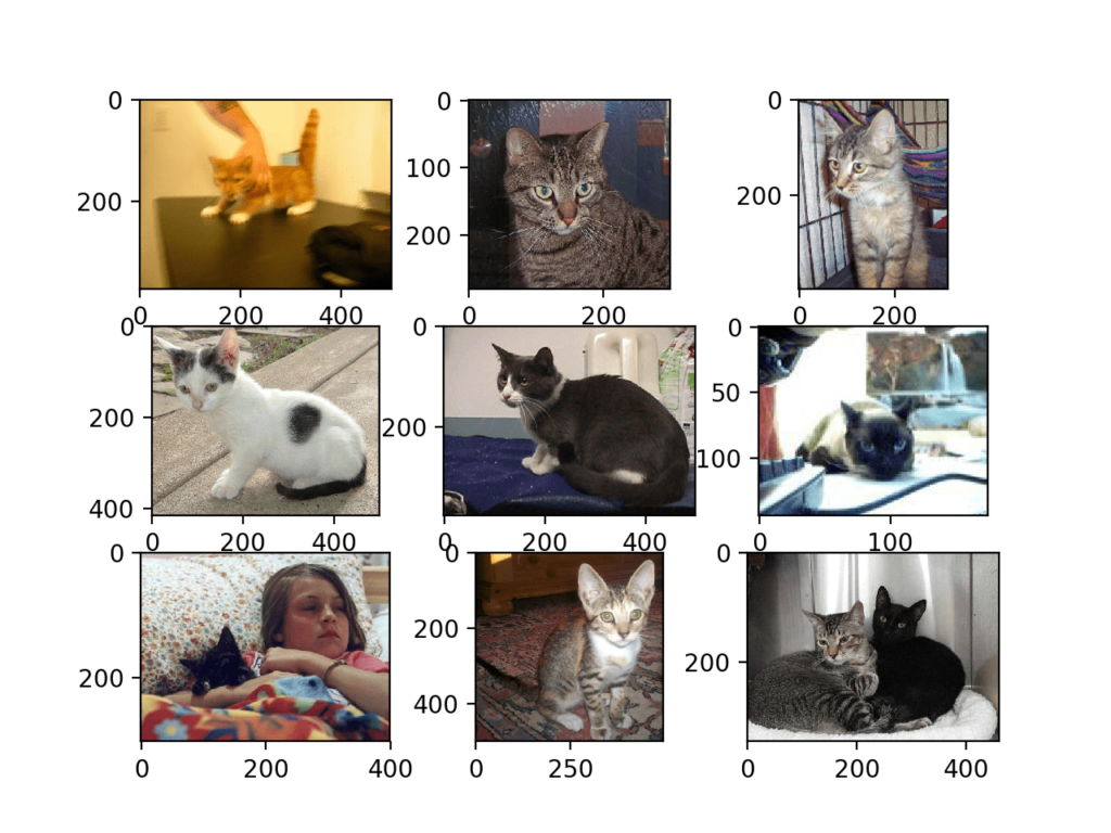
Plot of the first nine cat photos in the Dogs vs Cats dataset
Select a standard photo size
The photo must be reshaped before modeling so that all images have the same shape. This is usually a small square image.
There are many ways to achieve this, although the most common is a simple resize operation that stretches and distorts the aspect ratio of each image and forces it to turn into a new shape.
We can load all the photos and look at the distribution of the width and height of the photos, and then design a new photo size that best reflects what we are most likely to see in practice.
Smaller inputs mean that models can be trained faster, and often this concern governs the choice of image size. In this case, we will follow this method and choose a fixed size of 200×200 pixels.
Pre-processed photo size (optional)
If we want to load all the images into memory, we can estimate that it requires about 12 GB of RAM.
That’s 25,000 images, each with 200x200x3 pixels, or 3,000,000,000 32-bit pixel values.
We can load all the images, reshape them, and store them as a single NumPy array. This can fit the RAM on many modern machines, but not all, especially if you only have 8 GB to work with.
We can write custom code to load images into memory, resize them during loading, and then save them for modeling.
The following example uses the Keras image processing API to load all 25,000 photos in the training dataset and reshape them into 200×200 square photos. The tags are also determined based on the file name for each photo. Then save a set of photos and tags.
# load dogs vs cats dataset, reshape and save to a new file
from os import listdir
from numpy import asarray
from numpy import save
from keras.preprocessing.image import load_img
from keras.preprocessing.image import img_to_array
# define location of dataset
folder = 'train/'
photos, labels = list(), list()
# enumerate files in the directory
for file in listdir(folder):
	# determine class
	output = 0.0
	if file.startswith('cat'):
		output = 1.0
	# load image
	photo = load_img(folder + file, target_size=(200, 200))
	# convert to numpy array
	photo = img_to_array(photo)
	# store
	photos.append(photo)
	labels.append(output)
# convert to a numpy arrays
photos = asarray(photos)
labels = asarray(labels)
print(photos.shape, labels.shape)
# save the reshaped photos
save('dogs_vs_cats_photos.npy', photos)
save('dogs_vs_cats_labels.npy', labels)
Running the example may take about a minute to load all the images into memory and print the shape of the loaded data to confirm that it has loaded correctly.
Note: Running this example assumes that you have more than 12 GB of RAM. If you don’t have enough memory, you can skip this example; It is provided as a demonstration only.
(25000, 200, 200, 3) (25000,)At the end of the run, two files named “dogs_vs_cats_photos.npy” and “dogs_vs_cats_labels.npy” are created, which contain all the resized images and their associated class tags. Together, these files are only about 12 GB in size and load significantly faster than a single image.
The prepared data can be loaded directly; For example:
# load and confirm the shape
from numpy import load
photos = load('dogs_vs_cats_photos.npy')
labels = load('dogs_vs_cats_labels.npy')
print(photos.shape, labels.shape)
Preprocess photos into a standard catalog
Alternatively, we can use the Keras ImageDataGenerator class and the flow_from_directory() API to load the image step by step. This will be slower to execute, but will run on more machines.
The API prefers to split the data into separate train/ and test/ directories, each with a subdirectory for each class, e.g. a train/dog/ and a train/cat/ subdirectory, and the same goes for test. The images are then organized under subdirectories.
We can write a script to create a copy of the dataset with this preferred structure. We will randomly select 25% of the images (or 6,250) for the test dataset.
First, we need to create the following directory structure:
dataset_dogs_vs_cats
├── test
│   ├── cats
│   └── dogs
└── train
    ├── cats
    └── dogs
We can use the makedirs() function to create directories in Python and use loops to create dog/ and cat/ subdirectories for train/ and test/ directories.
# create directories
dataset_home = 'dataset_dogs_vs_cats/'
subdirs = ['train/', 'test/']
for subdir in subdirs:
	# create label subdirectories
	labeldirs = ['dogs/', 'cats/']
	for labldir in labeldirs:
		newdir = dataset_home + subdir + labldir
		makedirs(newdir, exist_ok=True)
Next, we can enumerate all the image files in the dataset and copy them to the dog/ or cats/ subdirectory depending on the file name.
In addition, we can randomly decide to keep 25% of the images in the test dataset. This is done consistently by fixing the seed of the pseudo-random number generator so that we get the same data split every time we run the code.
# seed random number generator
seed(1)
# define ratio of pictures to use for validation
val_ratio = 0.25
# copy training dataset images into subdirectories
src_directory = 'train/'
for file in listdir(src_directory):
	src = src_directory + '/' + file
	dst_dir = 'train/'
	if random() < val_ratio:
		dst_dir = 'test/'
	if file.startswith('cat'):
		dst = dataset_home + dst_dir + 'cats/'  + file
		copyfile(src, dst)
	elif file.startswith('dog'):
		dst = dataset_home + dst_dir + 'dogs/'  + file
		copyfile(src, dst)
The full code example is listed below, and it is assumed that you have extracted the images from the downloaded train.zip into train/ in the current working directory.
# organize dataset into a useful structure
from os import makedirs
from os import listdir
from shutil import copyfile
from random import seed
from random import random
# create directories
dataset_home = 'dataset_dogs_vs_cats/'
subdirs = ['train/', 'test/']
for subdir in subdirs:
	# create label subdirectories
	labeldirs = ['dogs/', 'cats/']
	for labldir in labeldirs:
		newdir = dataset_home + subdir + labldir
		makedirs(newdir, exist_ok=True)
# seed random number generator
seed(1)
# define ratio of pictures to use for validation
val_ratio = 0.25
# copy training dataset images into subdirectories
src_directory = 'train/'
for file in listdir(src_directory):
	src = src_directory + '/' + file
	dst_dir = 'train/'
	if random() < val_ratio:
		dst_dir = 'test/'
	if file.startswith('cat'):
		dst = dataset_home + dst_dir + 'cats/'  + file
		copyfile(src, dst)
	elif file.startswith('dog'):
		dst = dataset_home + dst_dir + 'dogs/'  + file
		copyfile(src, dst)
After running the example, you will now have a new dataset_dogs_vs_cats/ directory with a train/ and val/ subfolder and more dog/can cats/ subdirectories, exactly as designed.
Develop a baseline CNN model
In this section, we can develop a baseline convolutional neural network model for the dog vs. cat dataset.
The baseline model will establish a minimum model performance that all of our other models can be compared to, as well as a model architecture that we can use as a basis for research and improvement.
A good place to start is the general architectural principles of the VGG model. This is a good place to start because they achieved top performance in the ILSVRC 2014 competition, and the modular structure of the architecture is easy to understand and implement. For more details on the VGG model, see the 2015 paper “Very Deep Convolutional Networks for Large-Scale Image Recognition”.
The architecture involves stacking convolutional layers with small 3×3 filters, followed by the maximum pooling layer. Together, these layers form a block that can be repeated, where the number of filters in each block increases with the depth of the network, such as 32, 64, 128, 256 for the first four blocks of the model. The fill is used for the convolutional layer to ensure that the height and width shape of the output feature map match the input.
How does python identify cats and dogs? We can explore this architecture on the dog-versus-cat problem and compare models of this architecture with 1, 2, and 3 blocks.
Each layer is initialized with the ReLU activation function and He weights, which is generally a best practice. For example, you can define a 3-block VGG-style architecture in Keras, where each block has a convolution and pooling layer, as follows:
# block 1
model.add(Conv2D(32, (3, 3), activation='relu', kernel_initializer='he_uniform', padding='same', input_shape=(200, 200, 3)))
model.add(MaxPooling2D((2, 2)))
# block 2
model.add(Conv2D(64, (3, 3), activation='relu', kernel_initializer='he_uniform', padding='same'))
model.add(MaxPooling2D((2, 2)))
# block 3
model.add(Conv2D(128, (3, 3), activation='relu', kernel_initializer='he_uniform', padding='same'))
model.add(MaxPooling2D((2, 2)))
We can create a function called define_model() that will define a model and return that it is ready to fit into the dataset. You can then customize this function to define a different baseline model, such as a model version with 1, 2, or 3 VGG style blocks.
The model will be suitable for stochastic gradient descent, and we will start with a conservative learning rate of 0.001 and a momentum of 0.9.
The problem is a binary classification task that requires predicting a value of 0 or 1. An output layer with 1 node and sigmoid activation will be used, and the model will be optimized using a binary cross-entropy loss function.
Here’s an example of a define_model() function that uses a vgg-style block to define a convolutional neural network model for a dog vs. cat problem.
# define cnn model
def define_model():
	model = Sequential()
	model.add(Conv2D(32, (3, 3), activation='relu', kernel_initializer='he_uniform', padding='same', input_shape=(200, 200, 3)))
	model.add(MaxPooling2D((2, 2)))
	model.add(Flatten())
	model.add(Dense(128, activation='relu', kernel_initializer='he_uniform'))
	model.add(Dense(1, activation='sigmoid'))
	# compile model
	opt = SGD(lr=0.001, momentum=0.9)
	model.compile(optimizer=opt, loss='binary_crossentropy', metrics=['accuracy'])
	return model
It can be called as needed to prepare the model, for example:
# define model
model = define_model()
Next, we need to prepare the data.
This involves first defining an instance of an ImageDataGenerator that scales the pixel values to a range of 0-1.
# create data generator
datagen = ImageDataGenerator(rescale=1.0/255.0)
Next, you’ll need to prepare iterators for your training and test datasets.
We can use the flow_from_directory() function on the data generator and create an iterator for each train/ and test/ directory. We have to specify that the problem is a binary classification problem with the “class_mode” parameter and load an image with a size of 200×200 pixels via the “target_size” parameter. We fixed the batch size at 64.
# prepare iterators
train_it = datagen.flow_from_directory('dataset_dogs_vs_cats/train/',
	class_mode='binary', batch_size=64, target_size=(200, 200))
test_it = datagen.flow_from_directory('dataset_dogs_vs_cats/test/',
	class_mode='binary', batch_size=64, target_size=(200, 200))
We can then fit the model using the training iterator (train_it) and use the test iterator (test_it) as the validation dataset during training.
You must specify the number of steps to train and test the iterator. This is the number of batches that will make up a period. This can be specified by the length of each iterator and will be the total number of images in the training and test catalog divided by the batch size (64).
The model will fit into 20 epochs, which is a small amount of data that checks if the model can learn the problem.
# fit model
history = model.fit_generator(train_it, steps_per_epoch=len(train_it),
	validation_data=test_it, validation_steps=len(test_it), epochs=20, verbose=0)
Once fitted, the final model can be evaluated directly on the test dataset and classification accuracy can be reported.
# evaluate model
_, acc = model.evaluate_generator(test_it, steps=len(test_it), verbose=0)
print('> %.3f' % (acc * 100.0))
Finally, we can create a graph of the history collected during training stored in the “history” directory returned from the call fit_generator().
History contains the model accuracy and loss on the test and training datasets at the end of each epoch. The line graph of these metrics at the training period provides a learning curve that we can use to understand whether the model is overfitted, underfitted, or well-fitted.
The summary_diagnostics() function below takes the history directory and creates a single graph with a loss line chart and another line chart for accuracy. The drawing is then saved to a file, and the file name is based on the script name. This is helpful if we want to evaluate many variations of the model in different files and automatically create a line diagram for each variant.
# plot diagnostic learning curves
def summarize_diagnostics(history):
	# plot loss
	pyplot.subplot(211)
	pyplot.title('Cross Entropy Loss')
	pyplot.plot(history.history['loss'], color='blue', label='train')
	pyplot.plot(history.history['val_loss'], color='orange', label='test')
	# plot accuracy
	pyplot.subplot(212)
	pyplot.title('Classification Accuracy')
	pyplot.plot(history.history['accuracy'], color='blue', label='train')
	pyplot.plot(history.history['val_accuracy'], color='orange', label='test')
	# save plot to file
	filename = sys.argv[0].split('/')[-1]
	pyplot.savefig(filename + '_plot.png')
	pyplot.close()
We can combine all of this into a simple testing tool for testing model configurations.
Listed below are full python examples of identifying dogs and cats that evaluate a monoblock baseline model on a dog and cat dataset.
# baseline model for the dogs vs cats dataset
import sys
from matplotlib import pyplot
from keras.utils import to_categorical
from keras.models import Sequential
from keras.layers import Conv2D
from keras.layers import MaxPooling2D
from keras.layers import Dense
from keras.layers import Flatten
from keras.optimizers import SGD
from keras.preprocessing.image import ImageDataGenerator

# define cnn model
def define_model():
	model = Sequential()
	model.add(Conv2D(32, (3, 3), activation='relu', kernel_initializer='he_uniform', padding='same', input_shape=(200, 200, 3)))
	model.add(MaxPooling2D((2, 2)))
	model.add(Flatten())
	model.add(Dense(128, activation='relu', kernel_initializer='he_uniform'))
	model.add(Dense(1, activation='sigmoid'))
	# compile model
	opt = SGD(lr=0.001, momentum=0.9)
	model.compile(optimizer=opt, loss='binary_crossentropy', metrics=['accuracy'])
	return model

# plot diagnostic learning curves
def summarize_diagnostics(history):
	# plot loss
	pyplot.subplot(211)
	pyplot.title('Cross Entropy Loss')
	pyplot.plot(history.history['loss'], color='blue', label='train')
	pyplot.plot(history.history['val_loss'], color='orange', label='test')
	# plot accuracy
	pyplot.subplot(212)
	pyplot.title('Classification Accuracy')
	pyplot.plot(history.history['accuracy'], color='blue', label='train')
	pyplot.plot(history.history['val_accuracy'], color='orange', label='test')
	# save plot to file
	filename = sys.argv[0].split('/')[-1]
	pyplot.savefig(filename + '_plot.png')
	pyplot.close()

# run the test harness for evaluating a model
def run_test_harness():
	# define model
	model = define_model()
	# create data generator
	datagen = ImageDataGenerator(rescale=1.0/255.0)
	# prepare iterators
	train_it = datagen.flow_from_directory('dataset_dogs_vs_cats/train/',
		class_mode='binary', batch_size=64, target_size=(200, 200))
	test_it = datagen.flow_from_directory('dataset_dogs_vs_cats/test/',
		class_mode='binary', batch_size=64, target_size=(200, 200))
	# fit model
	history = model.fit_generator(train_it, steps_per_epoch=len(train_it),
		validation_data=test_it, validation_steps=len(test_it), epochs=20, verbose=0)
	# evaluate model
	_, acc = model.evaluate_generator(test_it, steps=len(test_it), verbose=0)
	print('> %.3f' % (acc * 100.0))
	# learning curves
	summarize_diagnostics(history)

# entry point, run the test harness
run_test_harness()
Now that we have a testing tool, let’s take a look at the evaluation of three simple baseline models.
Monolithic VGG model
The monolithic VGG model has a single convolutional layer with 32 filters, followed by a maximum pooling layer.
The define_model() function for this model is defined in the previous section, but is provided again below for completeness.
# define cnn model
def define_model():
	model = Sequential()
	model.add(Conv2D(32, (3, 3), activation='relu', kernel_initializer='he_uniform', padding='same', input_shape=(200, 200, 3)))
	model.add(MaxPooling2D((2, 2)))
	model.add(Flatten())
	model.add(Dense(128, activation='relu', kernel_initializer='he_uniform'))
	model.add(Dense(1, activation='sigmoid'))
	# compile model
	opt = SGD(lr=0.001, momentum=0.9)
	model.compile(optimizer=opt, loss='binary_crossentropy', metrics=['accuracy'])
	return model
Run this example by first printing the size of the training and test datasets, confirming that the datasets are loaded correctly.
The model is then fitted and evaluated, which takes about 20 minutes on modern GPU hardware.
Found 18697 images belonging to 2 classes.
Found 6303 images belonging to 2 classes.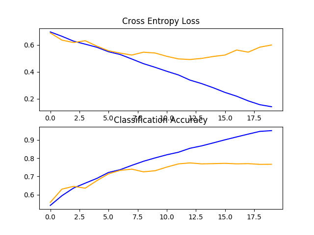
> 72.331Note: Your results may vary depending on the randomness of the algorithm or evaluation program or differences in numerical precision. Consider running the example multiple times and comparing the average results.
In this case, we can see that the model achieves about 72% accuracy on the test dataset.
A plot was also created showing the line plot of the loss and the accuracy of the model on the training (blue) and test (orange) datasets.
Looking at this graph, we can see that the model overfitted the training dataset at about 12 epochs.
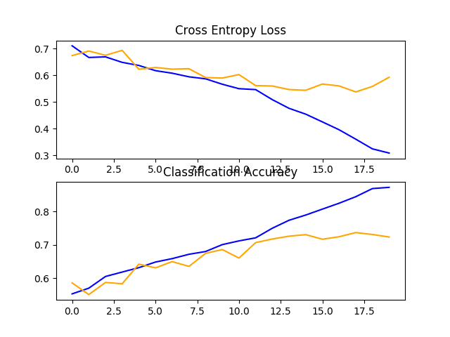
Line plot of the loss and accuracy learning curve of the baseline model with one VGG block on the dog and cat dataset
Categorizing photos of dogs and cats: two VGG models
The two-block VGG model expands the single-block model and adds a second block with 64 filters.
For the sake of completeness, the define_model() function for this model is provided below.
# define cnn model
def define_model():
	model = Sequential()
	model.add(Conv2D(32, (3, 3), activation='relu', kernel_initializer='he_uniform', padding='same', input_shape=(200, 200, 3)))
	model.add(MaxPooling2D((2, 2)))
	model.add(Conv2D(64, (3, 3), activation='relu', kernel_initializer='he_uniform', padding='same'))
	model.add(MaxPooling2D((2, 2)))
	model.add(Flatten())
	model.add(Dense(128, activation='relu', kernel_initializer='he_uniform'))
	model.add(Dense(1, activation='sigmoid'))
	# compile model
	opt = SGD(lr=0.001, momentum=0.9)
	model.compile(optimizer=opt, loss='binary_crossentropy', metrics=['accuracy'])
	return model
Running this example again will print the size of the training and test datasets, confirming that the datasets are loaded correctly.
Models are fitted and evaluated, and performance is reported on test datasets.
Found 18697 images belonging to 2 classes.
Found 6303 images belonging to 2 classes.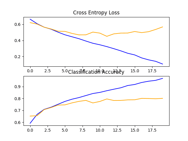
> 76.646Note: Your results may vary depending on the randomness of the algorithm or evaluation program or differences in numerical precision. Consider running the example multiple times and comparing the average results.
In this case, we can see that the model achieves a small increase in performance, from about 72% accuracy for one block to about 76% accuracy for two blocks
Looking at the learning curve graph, we can see that the model seems to be overfitting the training dataset again, perhaps faster, in this case, about 8 training periods.
This is most likely a result of an increase in model capacity, and we may expect this trend of faster overfitting to continue in the next model.
Line plot of the loss and accuracy learning curve of the baseline model with two VGG blocks on the dog and cat dataset
Three VGG models
The three-block VGG model expands on the two-piece model and adds a third block with 128 filters.
The define_model() function for this model is defined in the previous section, but is provided again below for completeness.
# define cnn model
def define_model():
	model = Sequential()
	model.add(Conv2D(32, (3, 3), activation='relu', kernel_initializer='he_uniform', padding='same', input_shape=(200, 200, 3)))
	model.add(MaxPooling2D((2, 2)))
	model.add(Conv2D(64, (3, 3), activation='relu', kernel_initializer='he_uniform', padding='same'))
	model.add(MaxPooling2D((2, 2)))
	model.add(Conv2D(128, (3, 3), activation='relu', kernel_initializer='he_uniform', padding='same'))
	model.add(MaxPooling2D((2, 2)))
	model.add(Flatten())
	model.add(Dense(128, activation='relu', kernel_initializer='he_uniform'))
	model.add(Dense(1, activation='sigmoid'))
	# compile model
	opt = SGD(lr=0.001, momentum=0.9)
	model.compile(optimizer=opt, loss='binary_crossentropy', metrics=['accuracy'])
	return model
Running this example will print the size of the training and test datasets, confirming that the datasets are loaded correctly.
Models are fitted and evaluated, and performance is reported on test datasets.
Found 18697 images belonging to 2 classes.
Found 6303 images belonging to 2 classes.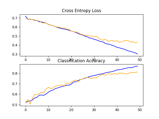
> 80.184Note: Your results may vary depending on the randomness of the algorithm or evaluation program or differences in numerical precision. Consider running the example multiple times and comparing the average results.
In this case, we can see that we have achieved a further improvement in performance, from about 76% with two blocks to about 80% accuracy with three blocks. This result is good because it is close to the state of the art using SVM reporting in the paper, with an accuracy rate of about 82%.
Looking back at the learning curve graph, we can see a similar trend of overfitting, in which case it may be delayed until period 5 or 6.
Line plot of the loss and accuracy learning curves of the baseline model with three VGG blocks on the dog and cat dataset
Discuss
We have explored three different models based on the VGG architecture.
The results can be summarized as follows, although given the randomness of the algorithm, we must assume that there are some differences in these results:
- VGG 1:72.331%
- VGG 2:76.646%
- VGG 3:80.184%
We’re seeing a trend of performance improving as capacity increases, but there are similar overfitting cases that are happening earlier and earlier in the run.
The results suggest that the model may benefit from regularization techniques. This may include techniques such as dropout, weight decay, and data augmentation. The latter can also improve performance by extending the training dataset to encourage the model to learn features that are further invariant to position.
Python’s method of identifying cats and dogs: developing model improvements
In the previous section, we developed a baseline model using the VGG style block and found a trend of performance improving as the model capacity increased.
In this section, we’ll start with a baseline model with three VGG blocks, i.e., VGG 3, and explore some simple improvements to the model.
Looking at the model’s learning curve during training, the model showed strong signs of overfitting. There are two ways we can explore to try to solve this overfit: dropout regularization and data augmentation.
Both methods are expected to slow down the rate of improvement during training and are expected to counter overfitting of the training dataset. Therefore, we increased the number of training epochs from 20 to 50 to provide more room for refinement for the model.
Dropout regularization
Dropout regularization is a computationally inexpensive way to regularize deep neural networks.
Dropout works by probabilitarily removing or “discarding” layers of inputs, which may be input variables in a data sample or activations from a previous layer. It has the effect of simulating a large number of networks with very different network structures, which in turn makes the nodes in the network generally more robust to inputs.
For more information about dropping out, see the post:
- How to use Dropout regularization in Keras to reduce overfitting
In general, a small number of dropouts can be applied after each VGG block, and more dropouts can be applied to the fully connected layer near the model output layer.
Here’s the define_model() function to add an updated version of the baseline model for dropout. In this case, a 20% dropout is applied after each VGG block, and a larger dropout rate of 50% is applied after the fully connected layer in the model classifier section.
# define cnn model
def define_model():
	model = Sequential()
	model.add(Conv2D(32, (3, 3), activation='relu', kernel_initializer='he_uniform', padding='same', input_shape=(200, 200, 3)))
	model.add(MaxPooling2D((2, 2)))
	model.add(Dropout(0.2))
	model.add(Conv2D(64, (3, 3), activation='relu', kernel_initializer='he_uniform', padding='same'))
	model.add(MaxPooling2D((2, 2)))
	model.add(Dropout(0.2))
	model.add(Conv2D(128, (3, 3), activation='relu', kernel_initializer='he_uniform', padding='same'))
	model.add(MaxPooling2D((2, 2)))
	model.add(Dropout(0.2))
	model.add(Flatten())
	model.add(Dense(128, activation='relu', kernel_initializer='he_uniform'))
	model.add(Dropout(0.5))
	model.add(Dense(1, activation='sigmoid'))
	# compile model
	opt = SGD(lr=0.001, momentum=0.9)
	model.compile(optimizer=opt, loss='binary_crossentropy', metrics=['accuracy'])
	return model
For the sake of completeness, the full code manifest for the baseline model is listed below, with dropouts added on the Dog vs. Cat dataset.
# baseline model with dropout for the dogs vs cats dataset
import sys
from matplotlib import pyplot
from keras.utils import to_categorical
from keras.models import Sequential
from keras.layers import Conv2D
from keras.layers import MaxPooling2D
from keras.layers import Dense
from keras.layers import Flatten
from keras.layers import Dropout
from keras.optimizers import SGD
from keras.preprocessing.image import ImageDataGenerator

# define cnn model
def define_model():
	model = Sequential()
	model.add(Conv2D(32, (3, 3), activation='relu', kernel_initializer='he_uniform', padding='same', input_shape=(200, 200, 3)))
	model.add(MaxPooling2D((2, 2)))
	model.add(Dropout(0.2))
	model.add(Conv2D(64, (3, 3), activation='relu', kernel_initializer='he_uniform', padding='same'))
	model.add(MaxPooling2D((2, 2)))
	model.add(Dropout(0.2))
	model.add(Conv2D(128, (3, 3), activation='relu', kernel_initializer='he_uniform', padding='same'))
	model.add(MaxPooling2D((2, 2)))
	model.add(Dropout(0.2))
	model.add(Flatten())
	model.add(Dense(128, activation='relu', kernel_initializer='he_uniform'))
	model.add(Dropout(0.5))
	model.add(Dense(1, activation='sigmoid'))
	# compile model
	opt = SGD(lr=0.001, momentum=0.9)
	model.compile(optimizer=opt, loss='binary_crossentropy', metrics=['accuracy'])
	return model

# plot diagnostic learning curves
def summarize_diagnostics(history):
	# plot loss
	pyplot.subplot(211)
	pyplot.title('Cross Entropy Loss')
	pyplot.plot(history.history['loss'], color='blue', label='train')
	pyplot.plot(history.history['val_loss'], color='orange', label='test')
	# plot accuracy
	pyplot.subplot(212)
	pyplot.title('Classification Accuracy')
	pyplot.plot(history.history['accuracy'], color='blue', label='train')
	pyplot.plot(history.history['val_accuracy'], color='orange', label='test')
	# save plot to file
	filename = sys.argv[0].split('/')[-1]
	pyplot.savefig(filename + '_plot.png')
	pyplot.close()

# run the test harness for evaluating a model
def run_test_harness():
	# define model
	model = define_model()
	# create data generator
	datagen = ImageDataGenerator(rescale=1.0/255.0)
	# prepare iterator
	train_it = datagen.flow_from_directory('dataset_dogs_vs_cats/train/',
		class_mode='binary', batch_size=64, target_size=(200, 200))
	test_it = datagen.flow_from_directory('dataset_dogs_vs_cats/test/',
		class_mode='binary', batch_size=64, target_size=(200, 200))
	# fit model
	history = model.fit_generator(train_it, steps_per_epoch=len(train_it),
		validation_data=test_it, validation_steps=len(test_it), epochs=50, verbose=0)
	# evaluate model
	_, acc = model.evaluate_generator(test_it, steps=len(test_it), verbose=0)
	print('> %.3f' % (acc * 100.0))
	# learning curves
	summarize_diagnostics(history)

# entry point, run the test harness
run_test_harness()
Run the sample first fits the model and then reports on the model’s performance on the maintained test dataset.
Note: Your results may vary depending on the randomness of the algorithm or evaluation program or differences in numerical precision. Consider running the example multiple times and comparing the average results.
In this case, we can see a slight improvement in model performance from about 80% accuracy of the baseline model to about 81% with dropouts added.
Found 18697 images belonging to 2 classes.
Found 6303 images belonging to 2 classes.
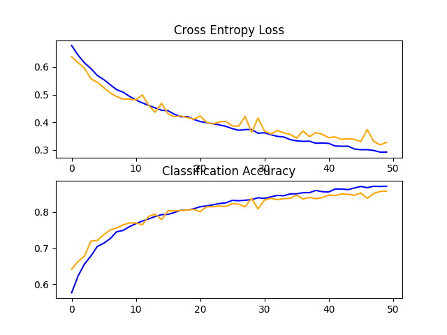
> 81.279Looking back at the learning curve, we can see that dropout has an impact on the rate of improvement of the model on both the training and test sets.
Overfitting has been reduced or delayed, but performance may start to stall at the end of the run.
The results suggest that further training periods may lead to further improvements in the model. In addition to the increase in training periods, it can also be interesting to explore that the dropout rate after the VGG block may be slightly higher.
Line plot of the loss and accuracy learning curve of the baseline model with dropout on the dog and cat dataset
Image data enhancement
Image data augmentation is a technique that can be used to artificially expand the size of a training dataset by creating a modified version of an image in a dataset.
Training a deep learning neural network model on more data can produce a more proficient model, while augmentation techniques can create variations of the image, improving the ability of the fitted model to generalize what they have learned to new images.
Data augmentation can also be used as a regularization technique to add noise to the training data and encourage the model to learn the same features without changing with their position in the input.
Making small changes to the input photos of dogs and cats may be useful to fix this issue, such as small movements and horizontal flips. These enhancements can be specified as parameters to the ImageDataGenerator used to train the dataset. Enhancements should not be used on test datasets because we want to evaluate the performance of the model on unmodified photos.
This requires us to have a separate instance of ImageDataGenerator for training and testing the dataset, followed by iterators for the training and testing sets created from the respective data generators. For example:
# create data generators
train_datagen = ImageDataGenerator(rescale=1.0/255.0,
	width_shift_range=0.1, height_shift_range=0.1, horizontal_flip=True)
test_datagen = ImageDataGenerator(rescale=1.0/255.0)
# prepare iterators
train_it = train_datagen.flow_from_directory('dataset_dogs_vs_cats/train/',
	class_mode='binary', batch_size=64, target_size=(200, 200))
test_it = test_datagen.flow_from_directory('dataset_dogs_vs_cats/test/',
	class_mode='binary', batch_size=64, target_size=(200, 200))
In this case, the photos in the training dataset will be enhanced with small (10%) random horizontal and vertical movements and random horizontal flips, creating a mirror image of the photos. The pixel values of the photos in the training and test steps are scaled in the same way.
Python Identification of Dogs and Cats Example – For completeness, a complete code checklist of baseline models with augmentation of training data for the dog and cat datasets is listed below.
# baseline model with data augmentation for the dogs vs cats dataset
import sys
from matplotlib import pyplot
from keras.utils import to_categorical
from keras.models import Sequential
from keras.layers import Conv2D
from keras.layers import MaxPooling2D
from keras.layers import Dense
from keras.layers import Flatten
from keras.optimizers import SGD
from keras.preprocessing.image import ImageDataGenerator

# define cnn model
def define_model():
	model = Sequential()
	model.add(Conv2D(32, (3, 3), activation='relu', kernel_initializer='he_uniform', padding='same', input_shape=(200, 200, 3)))
	model.add(MaxPooling2D((2, 2)))
	model.add(Conv2D(64, (3, 3), activation='relu', kernel_initializer='he_uniform', padding='same'))
	model.add(MaxPooling2D((2, 2)))
	model.add(Conv2D(128, (3, 3), activation='relu', kernel_initializer='he_uniform', padding='same'))
	model.add(MaxPooling2D((2, 2)))
	model.add(Flatten())
	model.add(Dense(128, activation='relu', kernel_initializer='he_uniform'))
	model.add(Dense(1, activation='sigmoid'))
	# compile model
	opt = SGD(lr=0.001, momentum=0.9)
	model.compile(optimizer=opt, loss='binary_crossentropy', metrics=['accuracy'])
	return model

# plot diagnostic learning curves
def summarize_diagnostics(history):
	# plot loss
	pyplot.subplot(211)
	pyplot.title('Cross Entropy Loss')
	pyplot.plot(history.history['loss'], color='blue', label='train')
	pyplot.plot(history.history['val_loss'], color='orange', label='test')
	# plot accuracy
	pyplot.subplot(212)
	pyplot.title('Classification Accuracy')
	pyplot.plot(history.history['accuracy'], color='blue', label='train')
	pyplot.plot(history.history['val_accuracy'], color='orange', label='test')
	# save plot to file
	filename = sys.argv[0].split('/')[-1]
	pyplot.savefig(filename + '_plot.png')
	pyplot.close()

# run the test harness for evaluating a model
def run_test_harness():
	# define model
	model = define_model()
	# create data generators
	train_datagen = ImageDataGenerator(rescale=1.0/255.0,
		width_shift_range=0.1, height_shift_range=0.1, horizontal_flip=True)
	test_datagen = ImageDataGenerator(rescale=1.0/255.0)
	# prepare iterators
	train_it = train_datagen.flow_from_directory('dataset_dogs_vs_cats/train/',
		class_mode='binary', batch_size=64, target_size=(200, 200))
	test_it = test_datagen.flow_from_directory('dataset_dogs_vs_cats/test/',
		class_mode='binary', batch_size=64, target_size=(200, 200))
	# fit model
	history = model.fit_generator(train_it, steps_per_epoch=len(train_it),
		validation_data=test_it, validation_steps=len(test_it), epochs=50, verbose=0)
	# evaluate model
	_, acc = model.evaluate_generator(test_it, steps=len(test_it), verbose=0)
	print('> %.3f' % (acc * 100.0))
	# learning curves
	summarize_diagnostics(history)

# entry point, run the test harness
run_test_harness()
Run the sample first fits the model and then reports on the model’s performance on the maintained test dataset.
Note: Your results may vary depending on the randomness of the algorithm or evaluation program or differences in numerical precision. Consider running the example multiple times and comparing the average results.
In this case, we can see a performance improvement of about 5%, from about 80% of the baseline model to about 85% of the baseline model, augmented with simple data.
> 85.816Looking back at the learning curve, we can see that the model seems to be able to learn further, with the loss of training and testing datasets still decreasing even at the end of the run. Experiments with 100 or more epochs are likely to yield better models.
It can be interesting to explore other enhancements that may further encourage learning to be invariant with their position in the input, such as small rotation and scaling.
Line plots of loss and accuracy learning curves with data-enhanced baseline models on dog and cat datasets
Discuss
We’ve explored three different improvements to the baseline model.
The results can be summarized as follows, although given the randomness of the algorithm, we must assume that there are some differences in these results:
- Baseline VGG3 + Dropout: 81.279%
- Baseline VGG3 + data augmentation: 85.816
As suspected, the addition of regularization techniques slows down the progress of the learning algorithm and reduces overfitting, which improves the performance of the retention dataset. The combination of the two methods with a further increase in the number of training periods may lead to further improvements.
This is just the beginning of the types of improvements that can be explored on this dataset. In addition to making adjustments to the described regularization methods, other regularization methods such as weight decay and early stop can be explored.
It may be worth exploring changes in learning algorithms, such as changes in learning rates, the use of learning rate plans, or adaptive learning rates, such as Adam.
Alternative model architectures may also be worth exploring. The baseline model selected is expected to provide more capacity than may be needed to address this issue, and smaller models may train faster, which in turn may result in better performance.
How does python identify cats and dogs? Explore transfer learning
Transfer learning involves using all or part of a model trained on a related task.
Keras provides a range of pre-trained models that can be loaded and used in whole or in part through the Keras application API.
A useful transfer learning model is one of the VGG models, such as VGG-16 with 16 layers, which achieved the highest score in the ImageNet photo classification challenge at the time of development.
The model consists of two main parts, the feature extractor part of the model consisting of VGG blocks, and the classifier part of the model consisting of a fully connected layer and an output layer.
We can use the feature extraction section of the model and add a new classifier section of the model, which is tailored to the dog and cat datasets. Specifically, we can keep the weights of all convolutional layers fixed during training and train only new fully connected layers that will learn to interpret the features extracted from the model and do binary classification.
This can be achieved by loading the VGG-16 model, removing the fully connected layer from the output of the model, and then adding a new fully connected layer to interpret the model output and make predictions. The classifier portion of the model can be automatically removed by setting the “include_top” parameter to “False“, which also requires that the model also specify the shape of the input, in this case (224, 224, 3). This means that the loaded model ends at the last maximum pooling layer, after which we can manually add a Flatten layer and a new classifier layer.
The define_model() function below achieves this and returns a new model ready to be trained.
# define cnn model
def define_model():
	# load model
	model = VGG16(include_top=False, input_shape=(224, 224, 3))
	# mark loaded layers as not trainable
	for layer in model.layers:
		layer.trainable = False
	# add new classifier layers
	flat1 = Flatten()(model.layers[-1].output)
	class1 = Dense(128, activation='relu', kernel_initializer='he_uniform')(flat1)
	output = Dense(1, activation='sigmoid')(class1)
	# define new model
	model = Model(inputs=model.inputs, outputs=output)
	# compile model
	opt = SGD(lr=0.001, momentum=0.9)
	model.compile(optimizer=opt, loss='binary_crossentropy', metrics=['accuracy'])
	return model
Once created, we can train the model on the training dataset as before.
In this case, a lot of training is not needed, as only the new fully connected layer and output layer have trainable weights. Therefore, we fixed the number of training epochs at 10.
The VGG16 model was trained on a specific ImageNet challenge dataset. As a result, it is configured to expect the input image to have a shape of 224×224 pixels. When loading photos from the dog and cat dataset, we will use it as the target size.
The model also wants the image to be centered. That is, the average pixel values for each channel (red, green, and blue) computed on the ImageNet training dataset are subtracted from the input. Keras provides a function to perform this preparation for a single photo via the preprocess_input() function. Nonetheless, we can achieve the same effect with the ImageDataGenerator by setting the “featurewise_center” parameter to “True” and manually specifying the average pixel value used when centering as the average of the ImageNet training dataset: [123.68, 116.779, 103.939] .
Python identification of dogs and cats example: The complete code list of VGG models for transfer learning on the dog and cat dataset is listed below.
# vgg16 model used for transfer learning on the dogs and cats dataset
import sys
from matplotlib import pyplot
from keras.utils import to_categorical
from keras.applications.vgg16 import VGG16
from keras.models import Model
from keras.layers import Dense
from keras.layers import Flatten
from keras.optimizers import SGD
from keras.preprocessing.image import ImageDataGenerator

# define cnn model
def define_model():
	# load model
	model = VGG16(include_top=False, input_shape=(224, 224, 3))
	# mark loaded layers as not trainable
	for layer in model.layers:
		layer.trainable = False
	# add new classifier layers
	flat1 = Flatten()(model.layers[-1].output)
	class1 = Dense(128, activation='relu', kernel_initializer='he_uniform')(flat1)
	output = Dense(1, activation='sigmoid')(class1)
	# define new model
	model = Model(inputs=model.inputs, outputs=output)
	# compile model
	opt = SGD(lr=0.001, momentum=0.9)
	model.compile(optimizer=opt, loss='binary_crossentropy', metrics=['accuracy'])
	return model

# plot diagnostic learning curves
def summarize_diagnostics(history):
	# plot loss
	pyplot.subplot(211)
	pyplot.title('Cross Entropy Loss')
	pyplot.plot(history.history['loss'], color='blue', label='train')
	pyplot.plot(history.history['val_loss'], color='orange', label='test')
	# plot accuracy
	pyplot.subplot(212)
	pyplot.title('Classification Accuracy')
	pyplot.plot(history.history['accuracy'], color='blue', label='train')
	pyplot.plot(history.history['val_accuracy'], color='orange', label='test')
	# save plot to file
	filename = sys.argv[0].split('/')[-1]
	pyplot.savefig(filename + '_plot.png')
	pyplot.close()

# run the test harness for evaluating a model
def run_test_harness():
	# define model
	model = define_model()
	# create data generator
	datagen = ImageDataGenerator(featurewise_center=True)
	# specify imagenet mean values for centering
	datagen.mean = [123.68, 116.779, 103.939]
	# prepare iterator
	train_it = datagen.flow_from_directory('dataset_dogs_vs_cats/train/',
		class_mode='binary', batch_size=64, target_size=(224, 224))
	test_it = datagen.flow_from_directory('dataset_dogs_vs_cats/test/',
		class_mode='binary', batch_size=64, target_size=(224, 224))
	# fit model
	history = model.fit_generator(train_it, steps_per_epoch=len(train_it),
		validation_data=test_it, validation_steps=len(test_it), epochs=10, verbose=1)
	# evaluate model
	_, acc = model.evaluate_generator(test_it, steps=len(test_it), verbose=0)
	print('> %.3f' % (acc * 100.0))
	# learning curves
	summarize_diagnostics(history)

# entry point, run the test harness
run_test_harness()
Run the sample first fits the model and then reports on the model’s performance on the maintained test dataset.
Note: Your results may vary depending on the randomness of the algorithm or evaluation program or differences in numerical precision. Consider running the example multiple times and comparing the average results.
In this case, we can see that the model achieves impressive results on the maintained test dataset, with a classification accuracy of about 97%.
Found 18697 images belonging to 2 classes.
Found 6303 images belonging to 2 classes.
> 97.636
Looking at the learning curve, we can see that the model fits the dataset quickly. It does not exhibit strong overfitting, although the results suggest that the extra capacity in the classifier and/or the use of regularization may be helpful.
This approach can make a number of improvements, including adding dropout regularization to the classifier portion of the model, and perhaps even fine-tuning the weights of some or all of the layers in the featuredetector portion of the model.
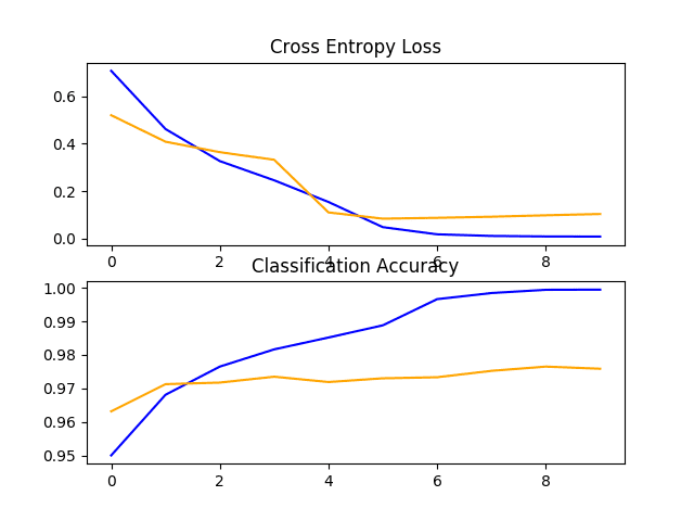
Line plot of the loss and accuracy learning curve of the VGG16 transfer learning model on the dog and cat dataset
How to complete the model and make predictions
As long as we have ideas, time, and resources to test them, the process of model improvement is likely to continue.
At some point, the final model configuration must be selected and adopted. In this case, we’ll keep it simple and use the VGG-16 transfer learning method as the final model.
First, we will finalize our model by fitting it on the entire training dataset and saving the model to a file for later use. Then we’ll load the saved model and use it to make predictions on a single image.
Classify photos of dogs and cats: Prepare the final dataset
The final model is typically suitable for all available data, such as a combination of all training and test datasets.
In this tutorial, we’ll demonstrate the final model that fits only on the training dataset, since we only have the labels of the training dataset.
The first step is to prepare the training dataset so that the ImageDataGenerator class can load it via the flow_from_directory() function. Specifically, we need to create a new directory that organizes all the training images into dog/ and cats/ subdirectories, without any separation into the train/ or test/ directories.
This can be done by updating the script we developed at the beginning of the tutorial. In this case, we will create a new finalize_dogs_vs_cats/ folder for the entire training dataset with dogs/ and cats/ subfolders.
The structure is as follows:
finalize_dogs_vs_cats
├── cats
└── dogs
For the sake of completeness, the updated script is listed below.
# organize dataset into a useful structure
from os import makedirs
from os import listdir
from shutil import copyfile
# create directories
dataset_home = 'finalize_dogs_vs_cats/'
# create label subdirectories
labeldirs = ['dogs/', 'cats/']
for labldir in labeldirs:
	newdir = dataset_home + labldir
	makedirs(newdir, exist_ok=True)
# copy training dataset images into subdirectories
src_directory = 'dogs-vs-cats/train/'
for file in listdir(src_directory):
	src = src_directory + '/' + file
	if file.startswith('cat'):
		dst = dataset_home + 'cats/'  + file
		copyfile(src, dst)
	elif file.startswith('dog'):
		dst = dataset_home + 'dogs/'  + file
		copyfile(src, dst)
Save the final model
How does python identify cats and dogs? We are now ready to fit the final model on the entire training dataset.
The flow_from_directory() must update all images loaded from the new finalize_dogs_vs_cats/directory.
# prepare iterator
train_it = datagen.flow_from_directory('finalize_dogs_vs_cats/',
	class_mode='binary', batch_size=64, target_size=(224, 224))
In addition, calls to fit_generator() no longer require specifying a validation dataset.
# fit model
model.fit_generator(train_it, steps_per_epoch=len(train_it), epochs=10, verbose=0)
Once fitted, we can save the final model to an H5 file by calling the save() function on the model and passing in the selected file name.
# save model
model.save('final_model.h5')
Please note that saving and loading Keras models requires the h5py library to be installed on your workstation.
Listed below is a complete python example of recognizing cats and dogs fitting the final model on a training dataset and saving it to a file.
# save the final model to file
from keras.applications.vgg16 import VGG16
from keras.models import Model
from keras.layers import Dense
from keras.layers import Flatten
from keras.optimizers import SGD
from keras.preprocessing.image import ImageDataGenerator

# define cnn model
def define_model():
	# load model
	model = VGG16(include_top=False, input_shape=(224, 224, 3))
	# mark loaded layers as not trainable
	for layer in model.layers:
		layer.trainable = False
	# add new classifier layers
	flat1 = Flatten()(model.layers[-1].output)
	class1 = Dense(128, activation='relu', kernel_initializer='he_uniform')(flat1)
	output = Dense(1, activation='sigmoid')(class1)
	# define new model
	model = Model(inputs=model.inputs, outputs=output)
	# compile model
	opt = SGD(lr=0.001, momentum=0.9)
	model.compile(optimizer=opt, loss='binary_crossentropy', metrics=['accuracy'])
	return model

# run the test harness for evaluating a model
def run_test_harness():
# define model
	model = define_model()
	# create data generator
	datagen = ImageDataGenerator(featurewise_center=True)
	# specify imagenet mean values for centering
	datagen.mean = [123.68, 116.779, 103.939]
	# prepare iterator
	train_it = datagen.flow_from_directory('finalize_dogs_vs_cats/',
		class_mode='binary', batch_size=64, target_size=(224, 224))
	# fit model
	model.fit_generator(train_it, steps_per_epoch=len(train_it), epochs=10, verbose=0)
	# save model
	model.save('final_model.h5')

# entry point, run the test harness
run_test_harness()
After running this example, you will now have a large 81 megabyte file named “final_model.h5” in your current working directory.
Make predictions
We can use our saved model to make predictions about new images.
The model assumes that the new images are in color and that they have been segmented so that one image contains at least one dog or cat.
Below are images taken from the test dataset of the dog and cat race. It doesn’t have a label, but we can clearly tell that it’s a picture of a dog. You can use the file name “sample_image.jpg” to save it in the
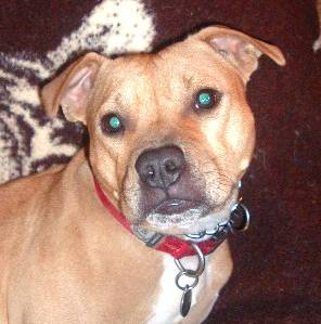
current working directory.
Dog (sample_image.jpg)
We’ll pretend it’s a brand-new, invisible image, prepared in the desired way, and see how we can use our saved model to predict the integer that the image represents. For this example, we expect class “1” for “Dog“.
Note: The subdirectories of the images, one for each class, are loaded alphabetically by the flow_from_directory() function, and an integer is assigned to each class. The subdirectory “cat” appears before “dog“, so the class tag is assigned an integer: cat=0, dog=1. This can be changed by calling the “classes” parameter in the flow_from_directory() when training the model.
How does python identify cats and dogs? First, we can load the image and force it to be 224×224 pixels. The loaded image can then be resized to include a single sample in the dataset. The pixel value must also be centered to match how the data is prepared during model training. The load_image() function achieves this, returning a loaded image ready for classification.
# load and prepare the image
def load_image(filename):
	# load the image
	img = load_img(filename, target_size=(224, 224))
	# convert to array
	img = img_to_array(img)
	# reshape into a single sample with 3 channels
	img = img.reshape(1, 224, 224, 3)
	# center pixel data
	img = img.astype('float32')
	img = img - [123.68, 116.779, 103.939]
	return img
Next, we can load the model as in the previous section and call the predict() function to predict the contents of the image as numbers between “0” and “1” for “cat” and “dog“, respectively.
# predict the class
result = model.predict(img)
The complete python example of recognizing cats and dogs is listed below.
# make a prediction for a new image.
from keras.preprocessing.image import load_img
from keras.preprocessing.image import img_to_array
from keras.models import load_model

# load and prepare the image
def load_image(filename):
	# load the image
	img = load_img(filename, target_size=(224, 224))
	# convert to array
	img = img_to_array(img)
	# reshape into a single sample with 3 channels
	img = img.reshape(1, 224, 224, 3)
	# center pixel data
	img = img.astype('float32')
	img = img - [123.68, 116.779, 103.939]
	return img

# load an image and predict the class
def run_example():
	# load the image
	img = load_image('sample_image.jpg')
	# load model
	model = load_model('final_model.h5')
	# predict the class
	result = model.predict(img)
	print(result[0])

# entry point, run the example
run_example()
Run the example first loads and prepares the image, loads the model, and then correctly predicts that the loaded image represents the “dog” or “1” class.
1Extend
Python’s Ways to Identify Cats and Dogs – This section lists some ideas for extended tutorials that you might want to explore.
- Adjust regularization. Explore subtle variations in the regularization techniques used on the baseline model, such as different loss rates and different image enhancements.
- Adjust the learning rate. Explore changes in the learning algorithms used to train the baseline model, such as alternative learning rates, learning rate plans, or adaptive learning rate algorithms such as Adam.
- Alternate pretrained models. Explore alternative pretrained models for transfer learning, such as Inception or ResNet, for this problem.
If you explore any of these extensions, I’d love to know.
Post your findings in the comments below.
Further reading
If you want to dig deeper, this section will provide more resources on the topic.
File
- Asirra: CAPTCHA for Manual Image Classification Using Interest Alignment, 2007.
- Machine Learning Attacks Against Asirra CAPTCHA, 2007.
- OverFeat: Integrated Identification, Localization, and Detection Using Convolutional Networks, 2013.
API
- Keras Application API
- Keras image processing API
- Keras Sequential Model API
Essay
- Dog vs Cat Kaggle Match.
- Dogs vs. Cats Redux: Kernel Edition.
- Dog vs Cat Dataset, Kaggle.
- Building Powerful Image Classification Models with Little Data, 2016.
Wraparound
How does python identify cats and dogs? In this tutorial, you learned how to develop a convolutional neural network to classify photos of dogs and cats.
Specifically, you learned:
- How to load and prepare photos of dogs and cats for modeling.
- How to develop a convolutional neural network for photo classification from scratch and improve model performance.
- How to develop a photo classification model using transfer learning.
Do you have any questions?
Ask your questions in the comments below and I’ll do my best to answer them.