ML: T Distributed Random Neighbor Embedding (t-SNE) algorithm

T-distributed random neighbour embedding (t-SNE) is a nonlinear dimensionality reduction technique, which is very suitable for embedding high-dimensional data in low-dimensional spaces in 2D or 3D for visualization.

What is Dimensionality Reduction?

Dimensionality reduction is a technique for representing 2- or 3-dimensional n-dimensional data (multidimensional data with many characteristics).

An example of dimensionality reduction can be discussed as a categorical problem, i.e., whether a student will play football or not, because both temperature and humidity depend on one feature because both features are highly correlated. As a result, we can reduce the number of features in such problems. 3-D classification problems can be difficult to visualize, while 2-D classification problems can be mapped to simple two-dimensional spaces, while 1-D problems can be mapped to simple lines.

How does t-SNE work?

t-SNE is a nonlinear dimensionality reduction algorithm that finds patterns in the data based on the similarity of data points with features, and calculates the similarity of points as the conditional probability that point A selects point B as its neighbor.

It then tries to minimize the difference between these conditional probabilities (or similarities) in high-dimensional and low-dimensional spaces to achieve a perfect representation of data points in low-dimensional spaces.

Spatiotemporal complexity

The algorithm calculates pairwise conditional probabilities and tries to minimize the sum of the probability differences in the higher and lower dimensions. This involves a lot of calculations and calculations. Therefore, the algorithm requires a lot of time and space to calculate. t-SNE has quadratic temporal and spatial complexity in the number of data points.

Apply t-SNE on the MNIST dataset

# Importing Necessary Modules.
import numpy as np
import pandas as pd
import matplotlib.pyplot as plt
from sklearn.manifold import TSNE
from sklearn.preprocessing import StandardScaler

Code 1: Read data

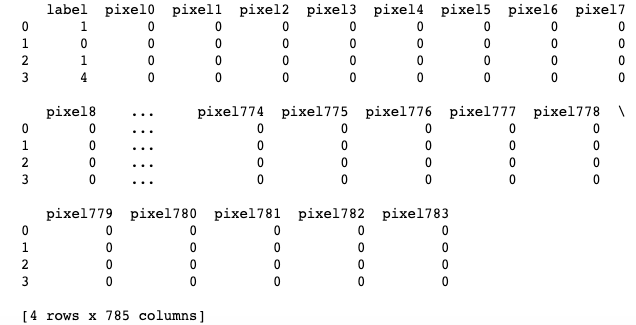
# Reading the data using pandas  
df = pd.read_csv( 'mnist_train.csv' )
  
# print first five rows of df
print (df.head( 4 )) 
  
# save the labels into a variable l.
l = df[ 'label' ]
  
# Drop the label feature and store the pixel data in d.
d = df.drop( "label" , axis = 1 )

The output is as follows:

Code 2:

Data preprocessing

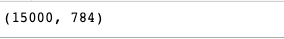
# Data-preprocessing: Standardizing the data
from sklearn.preprocessing import StandardScaler
  
standardized_data = StandardScaler().fit_transform(data)
  
print (standardized_data.shape)

The output is as follows:

Code 3:

# TSNE
# Picking the top 1000 points as TSNE
# takes a lot of time for 15K points
data_1000 = standardized_data[ 0 : 1000 , :]
labels_1000 = labels[ 0 : 1000 ]
  
model = TSNE(n_components = 2 , random_state = 0 )
# configuring the parameteres
# the number of components = 2
# default perplexity = 30
# default learning rate = 200
# default Maximum number of iterations
# for the optimization = 1000
  
tsne_data = model.fit_transform(data_1000)
  
  
# creating a new data frame which
# help us in ploting the result data
tsne_data = np.vstack((tsne_data.T, labels_1000)).T
tsne_df = pd.DataFrame(data = tsne_data, columns = ( "Dim_1" , "Dim_2" , "label" ))
  
# Ploting the result of tsne
sn.FacetGrid(tsne_df, hue = "label" , size = 6 ). map (
        plt.scatter, 'Dim_1' , 'Dim_2' ).add_legend()
  
plt.show()

The output is as follows:

First, your interview preparation enhances your data structure concepts with the Python DS course.

---